9.7. Sampling and Bootstrap Distributions of Parameters#
9.7.1. Animated and Interactive Examples of Sampling Distributions#
9.7.1.1. Sampling Distribution for Uniform \([0,10]\) Random Variable#
U= stats.uniform(0,10, )
sampling_dist(U, 'Uniform $[0,10]$')
9.7.1.2. Sampling Distribution for Exponential (\(\lambda=1/5\)) Random Variable#
E=stats.expon(scale=5)
sampling_dist(E, 'Exponential $\lambda=1/5$')
9.7.1.3. Sampling Distribution For Chi-Squared Random Variable with 6 Degrees of Freedom#
C=stats.chi2(df=6 )
sampling_dist(C, "Chi-Sq dof=6")
9.7.1.4. Sampling Distribution for Binomial Random Variable with 100 Trials and Probability of Success 0.2#
B = stats.binom(100, 0.2)
sampling_dist(B, "Binomial $(100,0.2)$")
9.7.1.5. Sampling Distribution for Average of Two Uniform Random Variables#
U= stats.uniform(0,10)
sampling_dist(U, "Uniform $[0,10]$")
9.7.1.6. Sampling Distribution for Average of Two Normal Random Variables#
N= stats.norm(3, 2)
sampling_dist(N, "Normal (0,1)")
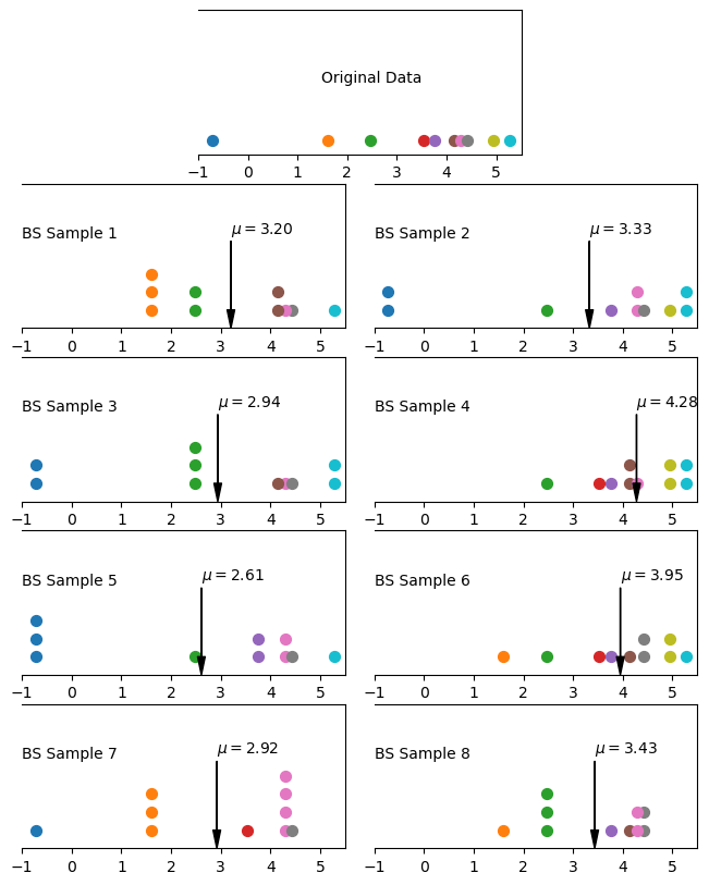
9.7.2. Code For Generating Images of Bootstrap Samples and Averages#
The code for generating the image of bootstrap samples and averages was omitted from the text. I am including it here:
import matplotlib.gridspec as gridspec
gs = gridspec.GridSpec(5, 4)
#gs.update(wspace=0.5)

fig = plt.figure()
fig.set_dpi(100)
fig.set_size_inches(8, 10)
np.random.seed(23341)
N=stats.norm(3,2)
nvals = N.rvs(10)
nvals.sort()
#plt.scatter(nvals, 0.01 *np.ones(10), s=50)
ax1 = plt.subplot(gs[0, 1:3])
for i, val in enumerate(nvals):
  ax1.scatter(val, 0.01 , s=50, c='C'+str(i))
ax1.set_ylim(0, 0.1)
ax1.set_xlim(-1, 5.5)
np.random.seed(1234512)


#ax = plt.gca()
ax1.spines['left'].set_visible(False)
ax1.get_yaxis().set_visible(False)
ax1.text(2.5, 0.05, 'Original Data',horizontalalignment='center',)

#ax1 = plt.subplot(gs[0, :2], )
#ax3 = plt.subplot(gs[1, 1:3])


for sample in range(1,9):
  #bs = npr.choice(nvals, len(nvals))
  bs = npr.choice(np.arange(0,len(nvals)), len(nvals))
  bsvals = nvals[bs]
  counts={}
  for val in bs:
    counts[val]=0
  xstart = 2*((sample+1) %2)
  ax = plt.subplot(gs[(sample+1) // 2, xstart:xstart+2])


  for val in bs:
    counts[val]+=1
    ax.scatter(nvals[val], 0.005*counts[val], s=50, c = 'C'+str(val))

  height = 0.01*(max(counts.values())+1)
  avg = bsvals.mean()
  #ax.scatter(avg, 0.005, marker='x')
  #ax.arrow(avg, height-0.01, 0, -height+0.01+0.005, head_width = 0.15, head_length=0.005 )
  ax.annotate(f'$\mu=${avg:0.2f}', xy=(avg, 0),  xycoords = 'data',
              xytext = (avg, 0.03),
              arrowprops=dict(facecolor='black', width=0.2, headwidth=5),
              horizontalalignment='left', verticalalignment='top',
  )
  ax.text(-1, 0.025, 'BS Sample '+str(sample),horizontalalignment='left',)

  ax.set_ylim(0, 0.04)
  ax.set_xlim(-1, 5.5)

  ax.spines['left'].set_visible(False)
  ax.get_yaxis().set_visible(False)
9.7.3. Terminology Review#
Use the flashcards below to help you review the terminology introduced in this chapter. \(~~~~ ~~~~ ~~~~\)