8.7. Histograms of Continuous Random Variables and Kernel Density Estimation#
Animation Illustrating Creating a Histogram By Dropping Blocks
Create 40 Normal random variables:
import scipy.stats as stats

N=stats.norm()
N40=N.rvs(size=40)
Here is an animated GIF showing a histogram of data from this distribution being created step by step:
Animation Illustrating Stacking Blocks Centered on Observed Value
We repeat the process that created the histogram above, but let the blocks be centered on the observed value (rather than fitting to some histogram bin). Then we let each part of the block drop to the lowest unfilled level:
Animation Illustrating Stacking Smooth Shapes on Observed Values
Now we replace the rectangular block with a smoother shape — a Normal pdf. The idea is that the smoother shapes should combine to create a smoother estimate of the pdf of the random variable from which the samples came.
Here is an aminated GIF showing this new type of histogram of the data being created step by step: